1•An atomic microscope
When looking up chemicals, in particular organic ones, we often see information like bond lengths and bond angles. Here is a short table of some typical bond lengths in organic molecules:
| Bond | Length (Å) |
|---|---|
| \(\ch{C\bond C}\) | \(1.54\) |
| \(\ch{C\dbond C}\) | \(1.34\) |
| \(\ch{C\bond H}\) | \(1.09\) |
| \(\ch{C\bond O}\) | \(1.43\) |
| \(\ch{O\bond H}\) | \(0.96\) |
How do we figure out these lengths? Visible light operates at wavelengths \(\sim 5000 \Ang\) (which is teal by the way), so it is way off from resolving these distances which are three orders of magnitude smaller.
The idea is simple. Use waves with much smaller wavelengths, like x-rays, which lie between \(0.1 \Ang\) and \(100 \Ang\). The resulting technique is called x-ray diffraction.
In this post we will explore the main ideas of the process with a concrete example: phenol \((\ch{C_6H_6O})\), which is simply a benzene ring with a hydroxyl (\(\ch{\bond OH}\)) on one carbon (doesn't matter which due to symmetry). Our data comes from Zenodo, which uses x-rays of wavelength around \(1.54 \Ang\), produced from atomic transitions in copper.
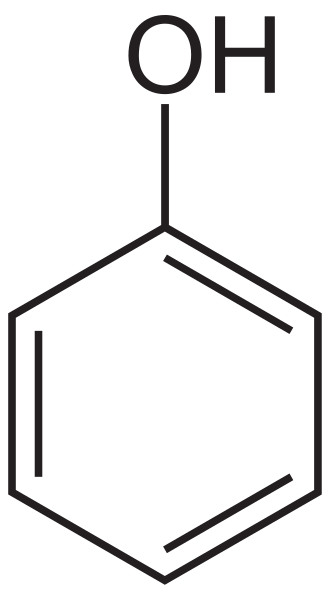
The structure of phenol. It is a benzene ring with a \(\ch{\bond OH}\) group.
By the end of this post, we will image the molecules of phenol, producing an picture like this.
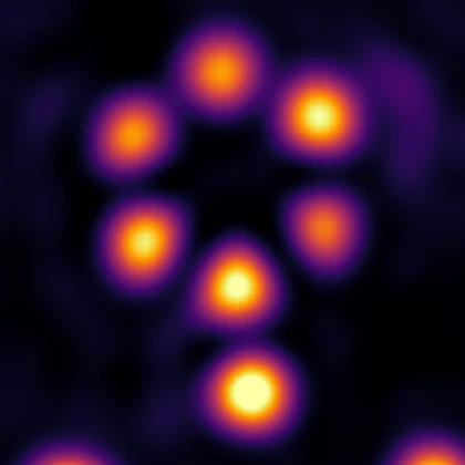
The result of imaging phenol with xray diffraction!
The broad steps are as follows:
- We hit a crystal of the target substance (here, phenol crystals) with x-rays of known wavelength in an x-ray diffractometer.
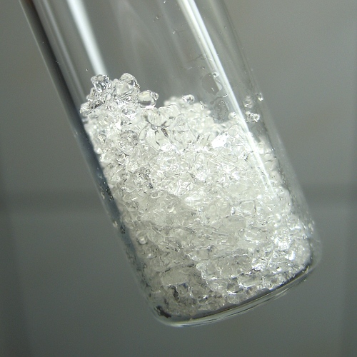
Phenol crystals. We use one of these crystals in the diffractometer.
- The x-rays scatter off the crystal electron densities. The resulting waves are also x-rays (due to elastic scattering). These scattered waves are detected by detectors mounted inside the diffractometer, placed in a grid of pixels.
A schematic of the Rigaku HyPix-Arc 100 diffractometer used to capture samples for the phenol crystal. It has two detector panels, positioned in this set up for the experiment. Note the shadow on the panels right where the \(\kin\) vector meets PANEL 1 on the right side. That area is supposed to have a very strong reflection, which is prevented by a manual cover, called a beamstop.
- Each pixel of the diffractometer counts incident photons to estimate the intensity at its location. This produces a frame of intensities which can be seen as an image:
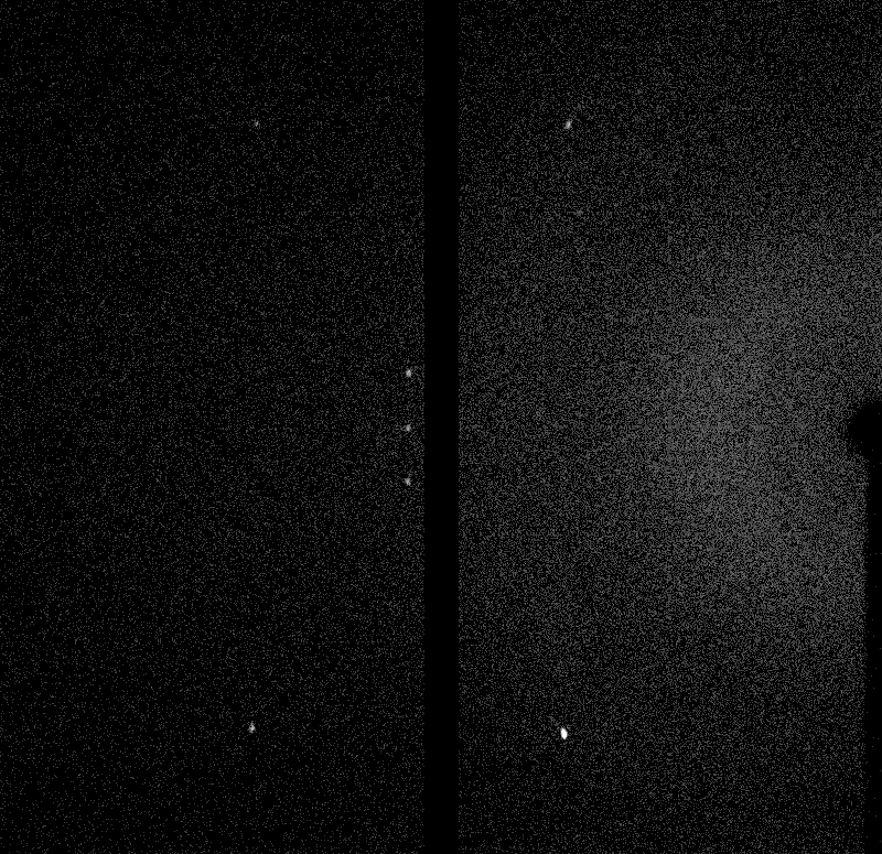
A raw frame of intensities. The diffractometer used has two panels. Observe the bright spots.
- Some locations display "spots" much brighter than the rest. In the setup above, we see at least seven. Five on the left pane and two on the right. We will soon see why these spots appear.
- We slowly rotate the crystal, hitting the crystal from many angles, and collect the frames.
- We analyze these frames and the spots, and hopefully it tells us something about the crystal's internal structure.
The point of this post is to see how we do step 6, the analysis. But to get to that, we will need to understand a bit of the physics1.
2•The physics involved
We begin with a closer inspection of the setup and the main actors.
2.1•X-rays are electromagnetic waves
A source of x-rays is simply a provider of incoming plane electromagnetic waves. The oscillating electric field can be written as (with \(j = \sqrt{-1}\))
where \(\k\) is the wavevector and \(\w\) is the angular frequency. These are related to the more familiar wavelength \(\lam\) and frequency \(\nu\) via the relations:
so that \(\w/k = \lam \nu = c \sim 3 \times 10^8 \met/\text{s}\), the speed of light in vacuum2.
Since \(\k\) is a vector, in addition to encoding the wavelength \(\lam\), it also represents the direction of the wave \(\hat{\k}\). Note that due to the relation \(\w/k = c\), the two quantities \((\hat{\k}, \lam)\) suffice to represent a plane wave.
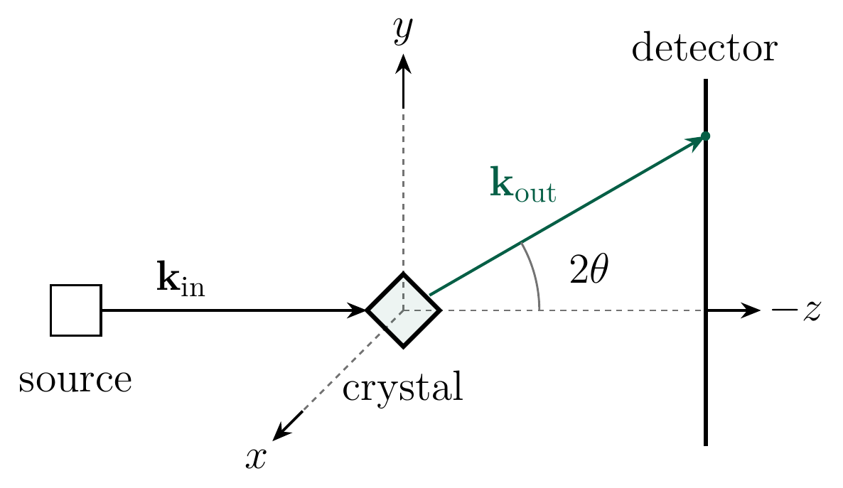
2D cross section of a simple diffractometer. The source produces x-rays \(\kin\) in the direction \(-z\) (this convention makes the detector plane have usual \(x-y\) coordinates). It hits the crystal at the origin and diffracts. We single out one direction \(\kout\) in which it hits the detector.
In a diffractometer (see the 3D setup or the 2D illustration above) we send x-rays from the source in the direction of \(\kin\), to hit the crystal sitting at the origin. The rays scatter elastically, i.e., without losing energy and thus still preserve their wavelength and remain x-rays. We consider a particular direction \(\kout\) such that the rays in that direction hit the detector.
But what exactly happens at that interaction between the rays and the crystal?
2.2•Scattering from electron density
Suppose our "scatterer" (like a crystal, or atom) is at the origin with density \(\eta(\br)\) (here \(\br\) is close to the origin), and consider a setup where the incoming wave is \(\kin\). The field of the radiation seen at a position \(\R = R \n\) is given by adding up the "contributions" for each crystal position \(\br\), and each "contribution" is a product of three terms:
The first two factors are \(\eta(\br)\) and \(e^{j\kin \cdot \br}\) (we omit the \(e^{-j\w t}\) time dependence by working in "Helmholtz space", see the footnote3). The third is the Green's function (essentially a PDE's response due to an impulse) of the Helmholtz equation in 3D, i.e. \(\frac{e^{jk|\R - \br|}}{|\R - \br|}\), up to constants. Therefore,
Of course, the hardest part of this derivation is to see why \(A(\R)\) should have that integral of products form above - we will not derive this, see here, eqns 3.8-3.10 for some details.
In our setups, \(R \gg |\br|\), since our detectors will be much farther than the extent of the crystal. For reference, we have \(R = 44 \mmet\) while the extent of the crystal is \(\sim 100 \umet\) (440x smaller). We are therefore justified in approximating
where the last step invokes \(\sqrt{1 - \eps} \approx 1 - \eps/2\) for small \(\eps\) and we neglect the \(|\br|^2/2R\) error. Substituting back into the expression for \(A\) we get
where we define \(\kout = k\n\) and the structure factor at \(\q = \kout - \kin\) as
which is just a Fourier transform of \(\eta\). Thus,
In practice, we cannot observe the true field \(A\) (frequency \(\nu \sim 10^{18}\)), but instead observe the averaged intensity \(I(\R) \propto |A(\R)|^2 \propto |F_\eta(\q)|^2\) via the number of photons detected by the detector. Note that we lose information about the phase of \(F_\eta\), and preserve just its magnitude.
The hope of x-ray crystallography is that this magnitude information is enough to reconstruct \(F_\eta\), and in turn by inverting the Fourier transform, \(\eta\). This is the task we have at hand.
2.3•The crystal structure
Nothing above required a crystal; the derivation holds for any electron density configuration. So why use crystals at all? After all, not everything crystallizes (glass never forms a lattice) and even where a crystal exists, it may not reflect its native structure, for instance α-synuclein in vivo.
The issue is disorder. Let us see how disorder kills any signal we can hope to get from our experiment. In a simple model, say each atom is located at some \(\br_i\) with \(i = 1, \ldots, N\). Further suppose that all of them were oriented in the same way, so that only the positions are disordered. If the electron density when a single atom is at the origin is \(\rho(\bs)\), the full density \(\eta\) is
with structure factor
And now disorder hits - since these \(\br_i\) are randomly scattered, the complex exponentials will just cancel each other, making each \(F_\eta(\q)\) completely noisy.
Crystals avoid this failure mode, since they are not only consistently ordered (but not at the level of each molecule, but only in small groups), but also consistently spaced. Let us see how this helps us.
In a crystal \(\eta\) is still a repeated copy of \(\rho\), but this time with ordered displacements \(\br_{hkl} = h \bb_1 + k \bb_2 + l \bb_3\) with \(h, k, l\) integers. Here \(\bb_1, \bb_2, \bb_3\) are the so-called crystallographic lattice vectors specifying a unit cell (with density \(\rho\)). The complete lattice is the collection of all such vectors
where we define the matrix \(B = [\bb_1, \bb_2, \bb_3]\). Note that due to the finite extent of the crystal, the crystal displacements are a large, but finite, subset of the full lattice. Regardless, our typical crystals have \(\sim 10^5\) cells in each dimension and therefore it will often be convenient to simply replace the crystal displacements with the full lattice, simplifying certain calculations.
A similar computation as earlier then yields:
Note that when \(\q^T B \h\) is a multiple of \(2\pi\), each \(e^{-j\q^T B \h} = 1\), thus all adding coherently. In practice, there are finite size effects which make it not scale with the number of cells, but it is still tremendously larger than the values for \(\q\) for which this condition is not satisfied. It is worth writing the \(\q^T B \h\) condition a bit better.
Fix \(\q\). Since \(\q^T B \h = (B^T \q) \cdot \h\), define \(\v = B^T \q\). Choosing \(\h\) to be the unit vectors, it is not hard to see that:
If \(\v \cdot \h\) is always an integer multiple of \(2\pi\) for all integer \(\h \in \Z^3\), that is, if \(\v \cdot \Z^3 \subseteq 2\pi \Z\), then \(\v\) has to be \(2\pi\) times an integer vector, i.e., \(\v \in 2\pi \Z^3\). The converse is also true (and obvious).
Going back to \(\q = (B^T)^{-1} \v\), we reach the equivalent condition4:
This is referred to as the reciprocal lattice of \(B\Z^3\). Note that the reciprocal of the reciprocal is the original lattice.
In conclusion, if the crystal lattice has the matrix \(B\), upon diffraction, we expect bright spots at \(\q\) belonging to the reciprocal lattice with matrix \(2\pi (B^T)^{-1}\). The wavelength \(\lam\) does not even enter this argument.
2.4•The raw data
Armed with this theory, we can start to discuss the data. In an x-ray diffractometer, the crystal is slowly rotated along an axis, recording the scattering pattern on the detector. Our particular diffractometer, the Rigaku HyPix-Arc 100 uses two panels instead of one (named panel 0 and panel 1), so we get two images for every fixed orientation of the crystal (two images per frame). Four different frames are shown below.
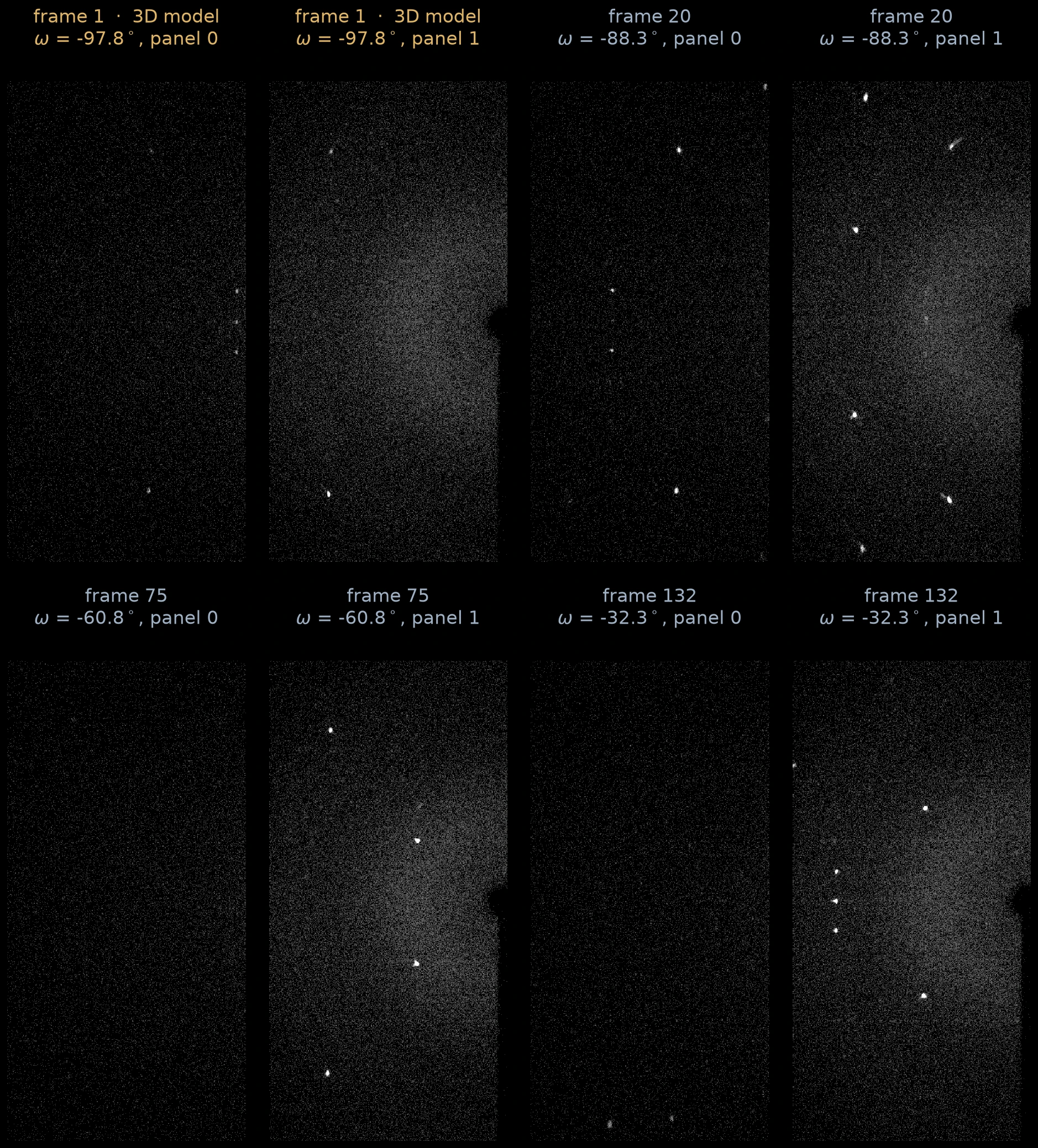
Raw panels from the x-ray diffractometer. Frame 1 on the top left consists of the two panels seen in the 3D model of the diffractometer.
Note the much brighter white spots, which correspond to the \(\q\) we derived in the previous section.
To understand the data a bit better, let us distinguish two frames of reference, both with (a fixed point on) the crystal as the origin: the lab frame, fixed to the lab, and the crystal frame fixed to the crystal.
Since the crystal rotates (say by a unitary matrix \(R\)), the effective \(\kin\) and possible \(\kout\) also rotate with the crystal. Thus for each \(R\), we capture a different "slice" of the possible \(\q = \kout - \kin\). Henceforth, all vectors will be in the crystal frame, and with some abuse of notation, we will continue to refer to the input and output wavevectors, in the crystal frame, as \(\kin\) and \(\kout\). For the four frames above, we illustrate below the (crystal frame) \(\q\) they sample.
Four frames above, converted to \(\q\)-space. Note that all these surfaces pass through \(\q = 0\). This is because not only is \(\kout = \kin\) possible physically, but, as you see from the diffractometer setup above, the \(\kin\) ray does intersect the detector panels (on the very right).
As we rotate the crystal, many \(\q\) are sampled multiple times (and some \(\q\) not at all). These frames, which are effectively photon counts recorded at that location, have to be "integrated", i.e., combined, to form an effective map of \(\q\)-space photon counts. It is not enough to simply average, the average must account for the estimated uncertainty (or stddev) of the counts, as well as eliminate background noise effects. It is also common to merge so-called Friedel pairs \(\q\) and \(-\q\), a consequence of the following simple fact known as Friedel's law:
Since \(\rho\) is real, the structure factor satisfies \(F_\rho(\q)^\star = F_\rho(-\q)\). In particular, \(|F_\rho(\q)| = |F_\rho(-\q)|\), that is, magnitudes cannot distinguish between \(\q\) and \(-\q\).
This is a significantly nontrivial task, especially due to the sensitivity of the situation under minor errors in the detector positions, rotation specifications etc. It is indeed possible to make some progress manually, but the task is best left to specialized software like DIALS, which I do here5. See the plot below for the final integrated data showing the \(\q\)-space locations for all the spots.
Plots from the data - notice the lattice structure. The sizes and colors indicate the recorded intensities at those spots.
Once this step is done, we are left with a collection of spots \(\q_1, \ldots, \q_n\), along with their recorded intensities, i.e., (proportional) estimates of \(|F_\rho(\q)|^2\), and we want to determine the structure \(\rho\).
3•Determining the crystal lattice
Our first task is to infer the structure of the crystal lattice, i.e., to determine \(\bb_1, \bb_2, \bb_3\). It will turn out that this stage does not require the intensity data (except the fact that the spots have high intensities, which is what made them "spots" in the first place).
We know the vectors \(\q_1, \ldots, \q_n\) come approximately (due to noise) from the reciprocal lattice \(2\pi(B^T)^{-1}\Z^3\). Let \(A = 2\pi(B^T)^{-1}\) for brevity. Then each \(\q_i \approx A\h_i\) for some integer vector \(\h_i \in \Z^3\). Recovering \(A\) would also recover \(B\), but how can we recover \(A\)?
The subtlety to observe here is that the choice of \(A\) is not unique due to the existence of nontrivial invertible matrices \(U\) which preserve \(\Z^3\), like
Replacing \(A\) by \(AU\) corresponds to replacing the columns \(\ba_1, \ba_2, \ba_3\) of \(A\) with \(\ba_1 - \ba_2, \ba_2, \ba_3\), clearly generating the same lattice.
Consequently, we will employ some aesthetics when choosing the lattice. The only hard constraints are that the three vectors \(\ba_1, \ba_2, \ba_3\) are linearly independent and generate the lattice. Our approach will prioritize choosing the basis with the smallest sidelengths.
A powerful approach to determining these lattice vectors is to consider the following score:
with equality (at least) at the origin \(\mathbf{0}\). If the \(\q_i\) were exactly \(A\h_i\) (i.e., no noise), then \(\q_i \cdot \bb = \h_i \cdot (A^T \bb)\). Once again, by the same logic as earlier, \(S(\bb)\) will be large if \(\bb \in 2\pi (A^T)^{-1} \Z^3\). This is the reciprocal lattice of \(A\Z^3\), which is already the reciprocal lattice of \(B\Z^3\)! Since the double reciprocal is simply the original, \(S(\bb) = 1\) if and only if \(\bb \in B\Z^3\).
In practice, noise attenuates the signal, so that such \(\bb\) have large scores but not the ideal 1. Regardless, we calculate this score on a very fine grid spanning \([-16, 16]^3 \Ang\), determine the local maximas, and plot them below.
Scatterplot of the peaks of score at least \(0.01\), with sizes showing their scores. There are a few tiny spurious peaks due to noise, but notice the prominent nodes. These are the true peaks showing the structure of the lattice.
An absolutely beautiful picture! Disregard the dust due to noise and discretization effects, but the large nodes exactly reproduce the structure of the crystal lattice6.
In fact, just by inspection near the origin, we can read off the lattice vectors:
in \(\Ang\).
To remove any small errors due to mesh discretization, we will slightly massage these chosen vectors by running a least-squares relaxation. For this, recall that the optimal \(B\) will satisfy \(\q_i^T B = 2\pi \h\) for some integer \(\h\) (this is because each \(\bb_{1/2/3} \cdot \q_i\) is supposed to be in \(2\pi \Z\)). An easy approach is therefore to (warm-) start with the chosen \(B\) above and minimize7:
A short computation leads to
in \(\Ang\) with lengths \(6.001, 8.970, 14.803 \Ang\) and angles \(89.93, 90.03, 89.88\) degrees. Essentially a cuboid8 with volume \(797 \Ang^3\).
The determined unit cell of the lattice.
With that, we have determined the unit cell of the crystal. Note that this calculation never used the intensities of the spots, just the fact that these spots showed up at all. The intensities will show up once we start trying to obtain the density \(\rho\).
4•The electron density
With the lattice structure in hand, we can finally focus on our true goal, the electron density.
4.1•Molecules per cell
Nothing above requires each cell to contain exactly one molecule. Our calculations merely establish that the overall electron density of the crystal, \(\eta\), is periodic with periodicity described by the lattice vectors above. Each unit of this periodicity, \(\rho\), can come from one or more molecules. However, one hopes that there are only a few molecules packed per cell. Otherwise their electron densities will be too crowded, and it will be hard to distinguish between them. Turns out we don't need to hope, there is a way to approximately see how many molecules there are in a cell.
The periodicity of the crystal implies that the mass density of a cell (distinct from the electron density) equals the mass density of the crystal, which is macroscopic and measurable! For phenol, Wikipedia lists9 it at \(1.07\) g/cm3. Given our cell volume of \(797 \Ang^3,\) this implies a per-cell mass of \(8.528 \times 10^{-22}\) g. Phenol weighs \(94.113\) g/mol, which is \(94.113 / N_A \approx 1.563 \times 10^{-22}\) g per molecule of phenol. The number of molecules per cell, \(Z\), is therefore
This is not exactly an integer like we had hoped, perhaps due to errors. At least it suggests that we can expect somewhere around 5 or 6 molecules per cell.
4.2•Normalizing to a unit cube
Recall from earlier that by counting photons, the instrument measures the intensities
where the last sum is over \(\h\) integer indices in the crystal. Assuming this to be the same for all the spots since \(\q\) is in the reciprocal lattice making \(\q^T B \h \in 2\pi \Z\), we are left with
Since each \(\R\) corresponds to a spot \(\q\), we will replace \(I(\R)\) with \(I(\q)\). In fact the square root of this (i.e., the amplitude \(|F_\rho(\q)|\)) was exactly what was plotted earlier in this figure. But we now know the matrix \(B\) such that \(\q \in 2\pi (B^T)^{-1} \Z^3\), which allows us to make the first steps towards reconstructing \(\rho\).
Substituting \(\q = 2\pi (B^T)^{-1}\h\) into the expression for \(F_\rho(\q)\) we get
Let \(\srho(\bs) = \rho(B\bs)\) be the cell-normalized density (because \(\br \to B\br\) sends \([0, 1]^3\) to the unit cell). Substituting \(\bs = B^{-1}\br\) the last expression reduces to
Since \(|\det B| \approx 797 \Ang^3\) is the known volume of the cell, we have
where we define the normalized observations
Our spot observations therefore effectively give us a table10 of \(|\sF(\h)|^2\) (where the \(\h\) correspond to the \(\q\)), and if we manage to obtain \(\srho\), we can scale it to obtain \(\rho\).
The one wrinkle is that even though apparently \(\sF\) is a Fourier transform of \(\srho\), its Fourier inverse \(\hrho\), calculated below, is not just \(\srho\) due to periodic effects.
that is, \(\hrho\) recovers the periodic sum of \(\srho\). Step \((\star)\) uses the following periodic delta identity:
see this answer for a proof. Regardless, \(\srho\) is typically highly localized near the atoms, which are inside the cell, so that the periodic extension does not matter, and we would recover \(\srho\)11.
We have reduced the problem to the following normalized variant that does not involve the shearing due to \(B\):
Given noisy observations proportional to \(|\sF(\h)| = \Abs{\displaystyle\int \srho(\bs) e^{-2\pi j \h \cdot \bs} \d\bs}\), for a large collection of \(h \in \Z^3\), reconstruct \(\srho\).
But of course, this reduction did not remove the essential difficulty of the problem, that is the lack of the phases of \(\sF\).
4.3•Charge flipping
Skipping almost the entire rich history12 of ideas to tackle this problem, we arrive at an almost magical approach proposed by G. Oszlányi and A. Süto (2004), called charge flipping.
For notational simplicity, we refer to \(\srho\) as \(\rho\) and \(\sF\) as \(F_\rho\) in this section.
Let us call the starting data \(A_\h\), which is supposed to be proportional to \(|F_\rho(\h)|\) (up to some noise). Charge flipping is an iterative algorithm. The key idea is to "shake" the estimated phases by flipping the sign on low density regions13. Since true atomic densities are mostly focused near atoms, this keeps the desired solution as an approximate fixed point.
We list the steps of charge flipping below, accompanied by planar cross-sections of the densities to illustrate the situation.
- Initialize: Start with a random assignment of the unknown phases, setting \(F_\h = A_\h e^{j\phi_\h}\), with \(\phi_\h\) uniform between \(0\) to \(2\pi\).
- Inverse Fourier: Compute the implied \(\srho\) via the sum above, on a fine enough14 \(n_1 \times n_2 \times n_3\) grid of points \(\br_1, \ldots, \br_N\) where \(N = n_1n_2n_3\).
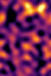
2D cross section of the density after random phases. Essentially meaningless due to the random phases.
Charge flipping: Flip the region where \(\srho\) is small. More precisely,
$$ \srho'(\br) = \begin{cases} -\srho(\br), & \text{if } \srho(\br) \lt \del, \\ \srho(\br), &\text{otherwise.} \end{cases} $$Choose \(\del = f \cdot \max \srho(\br)\), where \(f\) is some small tunable constant; we set \(f = 0.02\).
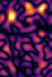
Charge flipped version of the cross section above. Note that the high positives were preserved, but one high negative area became positive.
Fourier back: Reconstruct \(G_\h\) by computing the following of the integral
$$ G_\h = \frac{1}{N} \sum \srho'(\br_j) e^{-2\pi j \h \cdot \br_j} \approx \int \srho'(\br) e^{-2\pi j \h \cdot \br} \d\br. $$Rescale to truth: The \(|G_\h|\) may not match the known \(A_\h\), so rescale to get
$$ F'_\h = \frac{G_\h}{|G_\h|} \cdot A_\h. $$- Repeat: Unless stable, go back to step 2 and repeat.
Density after step 2 in the next cycle. We iterate this process over and over again.
(If you are bothered with the subtleties of the fact that the inverse Fourier transform of \(\sF\) was not exactly \(\srho\), see the footnote11).
Here is a simulation of 806 cycles. Use the play button.
The charge flipping algorithm in action.
Magical! You see six distinct clusters of atoms pop up, each with 7 atoms. Those are the phenol molecules! Recall we had predicted there would be 5 or 6 per cell. By repeatedly shaking the phases and fixing their magnitudes, we are able to reach a valid solution. (We see 7 atoms, and not the full 13, because each hydrogen only has one electron next to a carbon, too hard to resolve at this resolution).
Now let us select one of those resolved molecules, and see how the density evolves in their plane.
The density in the molecular plane.
Do you see the six carbons and the oxygen? The oxygen is brighter because it has more electrons around it.
To end where we began, here are some estimates of geometric properties we get from the resolved structures, and how they compare to known values.
| Kind | Measured | Expected15 |
|---|---|---|
| aromatic \(\ch{C\bond C}\) | \(1.377 \pm 0.004 \Ang\) | \(1.390 \Ang\) |
| \(\ch{C\bond O}\) | \(1.375 \pm 0.012 \Ang\) | \(1.375 \Ang\) |
| \(\ch{C\bond C\bond C}\) angle | \(120.0^\circ \pm 0.02^\circ\) | \(120^\circ\) |
At which point you (if you started from zero) will know almost as much as I know.↩
In general, this is speed of light in the medium in which the system is immersed. In this case, we operate in vacuum or air, which have very similar speeds of light.↩
The Helmholtz equation is simply the wave equation when restricted to a fixed frequency (more technically, it is the Fourier transform of the wave equation in time). Our scattering is elastic, so we do not mix different frequencies (and thus, wavelengths), so it suffices to consider only a fixed \(\w\) equation, which makes Helmholtz the right fit.↩
Apparently it is common to use the notation \(B^{-T} = (B^T)^{-1}\). I cannot fault it too much since the operations are commutative: \((B^T)^{-1} = (B^{-1})^T\). Still, I am avoiding this here for clarity.↩
... after many failed attempts at matching their quality. It is one of those problems with many failure modes, and I fear, one that will take us somewhat farther from the main thread of the story. Although initially unwilling, I see the need for, and do gracefully accept, this magic hammer of DIALS.↩
There are two nodes close to zero. The lattice discretization was even, so there was nothing exactly at the origin, creating this split.↩
Since the starting \(B\) is already close to optimal, we alternate between rounding and minimizing the objective with fixed roundings.↩
Each crystal is of size \(\sim 0.1 \mmet\) on average (see the Zenodo listing) and the cell sidelength is \(\sim 10\Ang\), so we have \(\sim 10^{-4}/10^{-9} = 10^5\) cells on each side.↩
We are assuming our density is not too different from the state used on Wikipedia. Other sources (like here, see Table 1.1) list \(\sim 1.13\) g/cm3, yielding \(Z \sim 5.76\).↩
Our measured spots are proportional, not exactly equal, to \(|\sF(\h)|^2\).↩
In fact, due to the periodicity of \(\eta\) across the crystal, we can simply start with the assumption that our unit of periodicity, \(\rho\), is restricted to the unit cell. This is equivalent to working with \(\srho\) restricted to the unit cube, and would ensure that \(\hrho\) exactly a periodic copy of \(\srho\). In other words, \(\hrho\) restricted to the unit cube would be exactly \(\srho\).↩↩
For instance, the Patterson map, which uses the Fourier transform of \(|\sF|^2\) to determine the pairwise displacements, as well the direct methods of Hauptman-Karle (for which they received the 1985 Nobel prize in Chemistry), which determines relationships between phases due to the special structure of \(\rho\) as arising from electronic densities.↩
Note that this makes low positive density areas become low negative density, making it unphysical for a density.↩
Fine enough to avoid Nyquist aliasing. Since we have a bound on the observed \(\h\) per axis, it is sufficient to choose \(n_i > 2\max |\h_i|\). Our choices are much larger.↩
A. D. Fortes, Acta Cryst. E76 (2020) 1062–1069, doi:10.1107/S2056989020007719. See also CCDC 2474522.↩